Oscilloscope probes – why are they essential?

The article presents the most important, fundamental information and explains why 10:1 and 100:1 attenuating probes are commonly used during measurements, rather than 1:1 probes or ordinary pieces of cable. This article only provides the basics and a general, simplified approach – further explanations are given in subsequent articles.

Piotr Górecki – popularizer of electronics. Currently, he publishes his own magazine "Understanding Electronics". Previously, he was the Editor-in-Chief of a popular Polish magazine (Electronics for Everyone) for many years. He is also the author of hundreds of articles and educational projects. Until 1993, he worked in the telecommunications industry.

The development of technology means that digital oscilloscopes are becoming cheaper and have increasingly wider bandwidth. They seem to be ideal instruments due to digital processing, cursors, digital results of voltage, frequency, and time measurements. Unfortunately, quite often the measurement results obtained are unreliable. Very unreliable.

They are especially unreliable when connecting the oscilloscope alters the situation in the tested circuit. Certainly, the oscilloscope shows waveforms that are as true as possible, but occurring in the circuit after the oscilloscope has been connected, and does not show waveforms occurring during the normal operation of the circuit. It all depends on how much connecting the oscilloscope changes the situation in the circuit. This can be illustrated by a very simplified example shown in Figure 1. The tested circuit always has some internal resistance R_W (approximately).

Figure 1

At the same time, the oscilloscope has some input resistance R_I. There is no doubt that connecting the oscilloscope creates a voltage divider. The oscilloscope shows the voltage from such a divider, which is always lower than the voltage at point Y occurring during the normal operation of the circuit, without the additional load of the oscilloscope's input resistance R_I.

In general terms, the effective input resistance R_I of the oscilloscope should be much, even several times, larger than the internal resistance of the tested circuit or component. Then the error will be negligible. Even digital oscilloscopes are only seemingly very accurate. The amplitude measurement error is usually 2...4%. This leads to the conclusion that to avoid degrading the accuracy of the measurement, the oscilloscope's input resistance should be several tens of times, preferably at least 100 times greater than the effective internal resistance R_W of the tested circuit.

Beginner enthusiasts might think there is no problem because almost all oscilloscope inputs have high input resistance, equal to 1MΩ. Yes, the input resistance is usually 1 megaohm, but only resistance. And what is the impedance, that is, the resistance for variable waveforms?

After all, every oscilloscope, besides the relatively large resistance, also has some input capacitance – in better oscilloscopes slightly over 10pF, in worse even over 25pF.

Let's discuss this with an example: a 100-megahertz oscilloscope has a nominal input capacitance of about 18pF. With a ±3pF tolerance, its input can therefore have a round 20 picofarads. It seems little, but... what is the reactance and thus the impedance at a frequency of 100MHz?

From the formula XC = 1 / (2πfC), it is easy to calculate that for a capacitance of 20pF at 1kHz its reactance will be 8MΩ, and at 10kHz it will be 800kΩ. With further frequency increase, it will decrease and at 1MHz it will be 8kΩ, and at 100MHz only 80 ohms!

Yes! In a 100-megahertz oscilloscope, at the upper cutoff frequency of 100MHz, the input impedance is only 80Ω! That's not all: if we connect a cable as a probe to the oscilloscope input, the cable capacitance will be added to the oscilloscope's input capacitance as shown in Figure 2.

Figure 2

To a first approximation, we can assume that one meter of cable has a capacitance of about 80...100pF, depending on the type of cable. In parallel with the oscilloscope's input resistance R_I = 1MΩ, there will thus be at least 100pF capacitance. Notice that a capacitance of 100pF at 1MHz will have a reactance of 1.6 kilo-ohms, and at 100MHz only 16 ohms! At 250MHz, it will be less than 7 ohms! It therefore seems that at high frequencies, the impedance of the oscilloscope with such a probe will be purely capacitive reactance of negligible value, and the resistance R_I = 1MΩ can then be ignored.

The first problem is falsifying measurement results by creating a divider as indicated in Figure 1, because besides the actually large resistance R_I at high frequencies, there is also surprisingly very small capacitive reactance X_C.

The second problem is that during such measurement, we connect a relatively large total capacitance of the cable and oscilloscope to the tested circuit. How will this affect the operation of this circuit?

If it is, for example, a power supply circuit, then connecting a 100pF capacitance has no significance. But if it is, for example, a circuit of a generator with a quartz resonator or an LC circuit, connecting a 100pF capacitance will certainly disturb its operation and in many cases even make proper operation impossible. Even if the oscilloscope measures something, these will not be the waveforms occurring there during normal operation.

Figure 3

We are increasingly rarely testing delicate analog circuits and increasingly digital ones, where quite strong pulses with high frequency occur. Then a serious problem may arise, because according to the simplified Figure 3, adding the cable + oscilloscope capacitance of 100pF adds to the existing capacitances and increases the RC time constant, significantly slowing the digital signal depending on the output resistance RW (and the current capacity of the pulse source). Connecting a probe cable significantly changes the situation in the circuit and may cause errors in operation after connecting the oscilloscope. At best, there will be significant errors in measuring times and delays compared to those occurring during normal operation. Such measurements may turn out to be not only worthless but even misleading! The situation improves by increasing the input impedance of the oscilloscope, practically by reducing the capacitance of the probe and oscilloscope.

Capacitance Reduction

Someone might think that the measurement cable capacitance can be radically reduced by using two separate single wires, which during measurement can be spaced apart as shown in Figure 4.

Figure 4

Theoretically yes, but in practice it is a very bad idea. Indeed, the capacitance between two wires may then be small, but these long single wires become antennas picking up all kinds of "noise," both transmitted by electric and magnetic fields, because in total a loop is formed – a single-turn coil.

Not the way! If we use wires, they should be shielded cables, specifically "radio" coaxial, not microphone cables. In coaxial cables, the external shield is connected to ground and serves as protection, preventing the previously mentioned interference from entering the oscilloscope input.

Photo 5

Certainly, capacitance can be reduced by using the shortest possible measurement cables instead of probes, or even connecting the tested circuit directly to the BNC connector, as shown in the example in Photo 5. Then the load capacitance on the tested circuit will be practically equal to the oscilloscope input capacitance, about 20pF.

Can it be reduced? It turns out yes! And in several ways.

Here, less knowledgeable people need to be reminded that a variable voltage divider can be realized not only with two resistors but also using two capacitors, or possibly two coils (thus in Figure 1 the resistance markings were intentionally omitted). Different variants of 1:10 dividers are shown in Figure 6.

Figure 6

In any case, a 1:10 variable voltage divider can be realized using two series-connected capacitors as shown in Figure 6c. Their reactance will indeed change with frequency but proportionally, so the division ratio remains constant.

Now the reality: besides the input capacitance C_I and its frequency-dependent reactance X_C, the oscilloscope has an input resistance R_I of constant value. This creates some impedance Z_I. For the divider to work correctly, it should cooperate with an impedance of the same character but 9 times greater, which is easily achieved as shown in Figure 7a. What matters to us is that the capacitance CS in such a divider is 9 times smaller than the input capacitance C_I, and the effective input capacitance of the divider is only 1/10 of the capacitance C_I, as shown in Figure 7b. Such a configuration is often called a compensated voltage divider.

Figure 7

And here we have an unexpectedly simple way to reduce the input capacitance of the oscilloscope! Roughly, this is how oscilloscope probes work. A passive 1:10 oscilloscope probe contains a 9MΩ resistor and a compensating capacitor C_S, which theoretically should have 1/9 the input capacitance C_I of the oscilloscope.

The general rule is that to compensate such a divider, the RC time constants of the "upper" and "lower" branches must be equal, meaning: R_SC_S = R_I C_I.

In reality, it is more complicated. In different oscilloscopes, the capacitance C_I varies, usually from 10pF to 25pF, so the probe should have a variable capacitor – a trimmer – that allows precise adjustment of the 1:9 capacitance ratio.

Ideally, it should be connected in parallel with the 9MΩ resistor in the probe as shown in Figure 8a, which theoretically would allow obtaining the smallest input capacitance of the probe, on the order of 2pF.

Figure 8

For certain reasons, it is very often different: a fixed capacitor with an appropriate voltage rating is connected in parallel with the 9MΩ resistor, and the trimmer is connected to ground, in parallel with C_I , as shown in the simplified Figure 8b. This solution results in a somewhat larger input capacitance of the probe but is very often used.

The same rules apply to the 1:100 probe and divider, where according to Figure 9, theoretically, a 100MΩ resistance and input capacitance of only 0.2pF could be obtained.

Figure 9

Unfortunately, the last figures do not show the whole truth about probes. Additional capacitances come into play, not only mounting capacitances but especially the probe cable capacitance, which we did not account for in the figures. We can present a simplified (and as it will turn out in the next article, very inaccurate) equivalent circuit of a 1:10 probe as in Figure 10.

Figure 10

There it is very clear that considering the cable, the "lower" capacitance (C_I+ C_P) is on the order of 100pF. Even if a special low-capacitance cable for oscilloscope probes is used, it will still be several tens of picofarads.

Additionally, the capacitance of the probe tip to ground, marked as C_T (0.5...2pF) in Figure 10, contributes. This seriously changes the situation! In such a scenario, the total input capacitance of a 1:10 attenuating probe will probably not be less than 10pF, as Figure 11 indicates. It would be even worse if the compensation trimmer was connected "at the bottom," in parallel to C_P, C_I.

Figure 11

Sure, the oscilloscope with 1:10 probe will have an input resistance of 10MΩ, but due to the probe cable capacitance, it is difficult to achieve an input capacitance below 10pF. As a result, popular passive 1:10 probes have input capacitances on the order of a dozen picofarads, that is only a little less than the input capacitance of the oscilloscope itself without a probe.

Although with the divider we significantly reduced the influence of the probe cable, we are not completely satisfied. Much better is the case with passive 1:100 probes. Theoretically, without considering cable capacitance, they would allow input capacitance of about 0.2pF, but in practice because of the reasons given and others, their capacitance is significantly higher, usually on the order of 1...4pF.

One more detail: in the solution from Figure 9, in the 1:100 divider, we see a 99MΩ resistor, which would give an input resistance of 10MΩ, but this is not always optimal.

If not for a high-voltage probe, and when reducing capacitance is the key issue, input resistance equal to 100MΩ is usually not necessary. That is why many passive 1:100 probes have lower input resistance. A highly simplified example of a 1:100 probe with input resistance of 10MΩ and resistor R_S = 9.9MΩ is shown in Figure 12.

Figure 12

Such probes do not have to have a "round" input resistance of 10 or 100 megaohms – it can be different. And sometimes it is. In any case, frequency compensation is achieved when the RC time constants of the "upper" and "lower" RC circuits are equal, as illustrated in Figure 13.

Figure 13

"At the bottom" there is a parallel connection of resistances 111kΩ and 1MΩ, which gives an effective "lower" resistance of 99.91kΩ, practically 100kΩ. If there was no cable capacitance C_P, the "lower" capacitance would be 20pF, giving a "lower" time constant of 2μs. To obtain the same time constant with the "upper" resistance of 9.9MΩ, the compensating capacitance C_S should be 0.202pF.

If we more realistically assume that the "lower" capacitance in the probe with the cable is 100pF, then the "lower" time constant will be 10μs. To be the same "at the top," the capacitance C_S will be 1.01pF, but the total input capacitance of such probe will be higher due to the presence of mounting capacitances C_T (around 1pF).

Using such compensated dividers in probes, besides reducing input capacitance, has another important advantage: only a small fraction of the tested voltage is supplied to the oscilloscope input. This allows measuring voltages much higher than permissible at the oscilloscope input, provided the probe elements can withstand it. On the other hand, when measuring very small signals, the presence of a divider – attenuator is a significant disadvantage, as signals attenuated by it may simply disappear in the oscilloscope's internal noise, which is naturally rather high. We can return to these issues later.

Practical Conclusions

Today, popular oscilloscopes come with probes with a 1:1 / 1:10 switch. Figure 14 shows a simplified circuit of such a passive probe with switch S1.

Figure 14

Figure 15 shows the parameters of a 300-megahertz GW Instek probe. Here a surprise for less knowledgeable people may be the bandwidth in the 1:1 setting – only 10 megahertz!

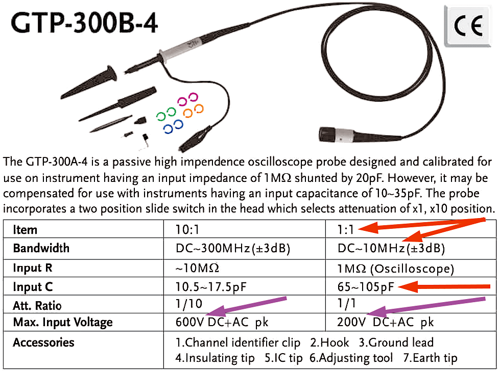
Figure 15

In other similar specifications, even smaller values are often found here, for example only 6MHz! This is no surprise since in this setting we only have a high-capacitance measurement cable, at least several tens of picofarads, often over 100pF. Together with the oscilloscope input capacitance C_I , this often exceeds 100pF, and thus there is very low reactance at higher frequencies. This is why the useful bandwidth is limited at the 1:1 setting.

The second surprise in Figure 15 may be the low allowable voltage in the 1:1 position – only 200V peak voltage (DC+AC), less than the allowable voltage of many oscilloscopes. The given voltages concern DC and slowly varying voltages. With increasing frequency, the allowable voltages are even lower – we can also return to this topic. In any case, we already see that at higher frequencies, using the probe in the 1:10 position makes sense only. Then the probe must be compensated, i.e., balance the frequency response of the probe using the built-in trimmer (the trimmer setting does not affect the 1:1 range).

Photo 16

In practice, probe compensation is done very simply using a low-frequency square wave signal. Every real oscilloscope has a built-in such calibration generator. The probe tip (1:10 or 1:100) should be touched to such output (example in Photo 16), and then, observing the waveform on the screen, adjust the trimmer so that the waveform most closely resembles a square – Figure 17. Such calibration only needs to be done once when connecting a given probe for the first time to a particular oscilloscope. After connecting it to another oscilloscope (with a different capacitance C_I ), calibration should be repeated.

Figure 17

The vast majority of probes have one trimmer for compensation using a low-frequency square wave of about 1kHz. However, some probes have two trimmers, the second for compensation in the highest frequency range using a square wave around 1MHz.

To summarize: the oscilloscope's input capacitance, especially the cable capacitance, drastically lowers input impedance at higher frequencies. Using a compensated divider, specifically an oscilloscope probe, significantly improves this situation. For various reasons, 1:10 probes are commonly used, while 1:100 probes are much less popular, and 1:1000 probes even less so. A key practical conclusion is: for most measurements, the oscilloscope should be used with a 1:10 probe, not a 1:1 probe.

The very important topics discussed do not exhaust the subject of oscilloscope probes. This is only an elementary introduction, the tip of the iceberg that does not touch on the most serious problems. In the next article – Secrets of Oscilloscope Probes – we will provide further surprising details. ©
Piotr Górecki

Transfer Multisort Elektronik (TME) is one of the world’s largest global distributors of electronic components, electrotechnical parts, workshop equipment, and industrial automation. The catalog includes over 1,500,000 products from 1,300 leading manufacturers. TME’s modern logistics centers in Łódź and Rzgów (Poland), with a combined area of over 40,000 m², ship nearly 6,000 packages daily to customers in more than 150 countries.

TME also invests in the development of knowledge and skills of young engineers and electronics enthusiasts through the TME Education project, and supports the tech community by organizing the TechMasterEvent series, promoting innovation and experience exchange.